I was recommended Hadley Wickham’s talk The Joy of Functional Programming (for Data Science) when I was struggling to code some iterative processes (you can find his talk on YouTube). The issue I ran into was trying to run row-wise and column-wise functions using for loops in R (a kerfuffle I’ll document in another blog post), which can get quite nasty with nested for loops.
The main lesson I learnt from the talk is: some clever programmers have wrapped up for loops in a function, map, that makes writing and reading code so much easier. It takes a while to get used to implementing these functions, but I can already say (in my very short two weeks of using it) that it’s a game-changer for my workflow. I think the main advantage of using map (and its cousins, which you can explore from the purrr package) is that it allow us to focus on both the action and the object whilst programming. In comparison, whilst using for loops I find myself focusing more on the object and the action can get lost. Here’s an example to show you what I mean:
# For loop approach:
out1 <- vector("double", ncol(mtcars))
for (i in seq_along(mtcars)) {
  out1[[i]] <- mean(mtcars[[i]], na.rm = TRUE)
}

out2 <- vector("double", ncol(mtcars))
for (i in seq_along(mtcars)) {
  out2[[i]] <- median(mtcars[[i]], na.rm = TRUE)
}

# Functional programming approach:
library(purrr)

out1 <- map_dbl(mtcars, mean, na.rm = TRUE)
out2 <- mtcars %>% map_dbl(median, na.rm = TRUE)

# Where map_dbl is an extension of map, returning
# a vector in double ('dbl') type.
You only figure out which actions we’re taking (calculating the mean and median) a few lines down the for loop, after the object has been defined. There is also more room for error as we have to define the object before we run the action every time (i.e. creating the vector and sequencing along each column before calculating the mean and median). The functional programming approach is more concise. You can also see that map plays well with the pipe.
Something to note: in the example above, we use map_dbl instead of just map. This is one of the many extensions to the map function; there is also map_chr to return character-type lists.
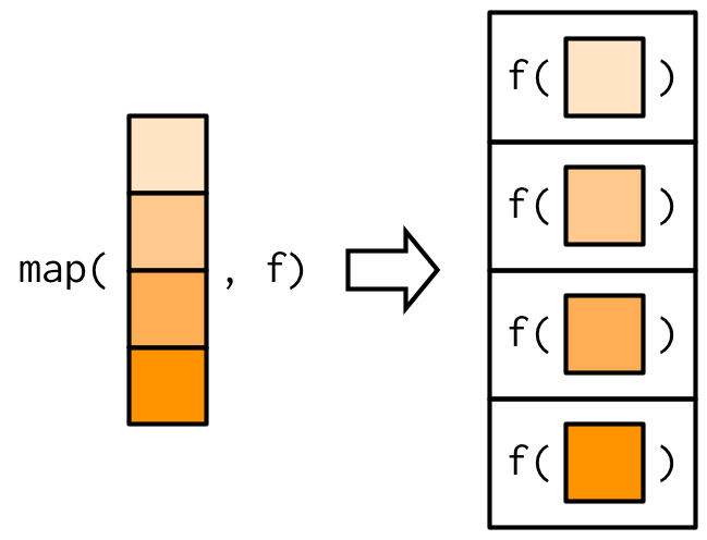
I also find the following figure handy to understand how the map functions work:

map function in R. Figure from Hadley Wickham’s Advanced R.Another thing to note is there are several ways of writing out the same thing using map. In the following bit of code you’ll find four different ways of writing out the same function: finding the number of unique values in each column of the mtcars dataset.
map_dbl(mtcars, function(x) length(unique(x)))

map_dbl(mtcars, ~ length(unique(.x)))

map_dbl(
  .x = mtcars,
  .f = length(unique(.x))
)

map_dbl(
  .x = mtcars,
  .f = \(x) length(unique(x))
)

# All three above returns:
#> mpg  cyl disp   hp drat   wt qsec   vs   am gear carb
#>  25    3   27   22   22   29   30    2    2    3    6
It took me a while to figure out when I needed to add a dot to the variable (.x)–and to be honest, I still haven’t gotten to the bottom of why we sometimes need to prefix x with a dot (and sometimes not).
Here’s another simple example, with an equivalent in lapply:
map(paths, ~ read.csv(.x))

# Equivalent to the following:
lapply(paths, function(x) read.csv(x))
Concise and easy to read.
The main issue I had with learning this concept was the steep learning curve. You have to put quite a bit of time into learning which functions are available in the purrr package. I still struggle with figuring out which function I should use and how I should write out the program. But as with most R packages, there are good resources out there that explains these functions really well. So despite the difficulties, I’ll be replacing most of my for loops with map.
Useful links for further reading:
- You can find the
purrrwebsite here. purrrhas a cheat sheet (released by RStudio) here.- Hadley Wickham gives a good explanation of this in Section 9.2 of his Advanced R textbook.